Correlation models and hypothesis testing
This demo shows how to use the PCMPy toolbox to test hypotheses about the true (noisefree) correlation between activity patterns as described in Diedrichsen et al. (2026). We will show how to obtain individual and group-level maximum-likelihood estimates of the true correlation between activity patterns, and how to test hypotheses about the size of these correlations using a bootstrap approach. In the first part of this jupyter notebook, we will focus on the single-pattern setting, in which we want to estimate the correlation between two activity patterns. In the second part, we will consider a slightly more complex multi-pattern setting, in which we want to estimate the true correlation between two sets of activity patterns measured under two different conditions.
[1]:
# First import necessary libraries
#(make sure PcmPy is in your python path)
import PcmPy as pcm
import numpy as np
import pandas as pd
import matplotlib.pyplot as plt
import seaborn as sns
from numpy import exp, sqrt
import scipy.stats as sps
Single pattern setting: Estimating the correlation between two patterns
The correlation between two activity patterns in fMRI can be quite low, even if the correspondence between these two patterns is perfect. This is because both patterns are measured with measurement noise. To solve this problem, we can obtain the maximum-likelihood estimator of the correlations, using repeated measurements of the same two activity patterns across multiple runs (repetitions) to estimate the signal and noise variance on each pattern. Note that this estimator is not unbiased, and can get unstable for very low signal to noise datasets - so we need to be caseful in the interpretation and inference (see Diedrichsen et al., 2026 for details).
In the simplest case of 2 activity patterns, the model will have 3 model parameters:
\(\sigma^2_x\): The strength (variance across voxels) of the activity patterns associated with condition X.
\(\sigma^2_y\): The strength (variance across voxels) of the activity patterns associated with condition Y.
\(r\): The true correlation between A and B
And one additional noise parameter:
\(\sigma^2_{\epsilon}\): The variance of the measurement noise across repeated measures of the same pattern.
To ensure that the variance parameters are positive, and the correlation between \(-1,1\), we fit the following nonlinear transforms:
\(\theta_1 = log(\sigma^2_x)\)
\(\theta_2 = log(\sigma^2_y)\)
\(\theta_3 = atanh(r)\)
\(\theta_{\epsilon} = log(\sigma^2_{\epsilon})\)
These (hyper-)parameters are collectively referred to by \(\theta\) (thetas). The algorithm maximizes the Type-II maximum likelihood of the data given the parameters: \(p(Y|\theta)\)
Simulating data
In this example, we will use simulated data with a known correlation between the true (noiseless) activity patterns (Mtrue). In this example, we set that our two activity patterns are positively correlated with a true correlation of 0.7.
Note that in the single-pattern setting, we crate a
pcm.CorrelationModelwithnum_itemsset to 1, as we have only 1 activity pattern per condition. We also setcond_effecttoFalse, as we do not want to account for the overall condition effect.
Because the correlation of the true mode (Mtrue) is fixedm the model has only 2 hyper-parameters reflecting the signal strength (or true pattern variance) for each activity pattern (item).
[2]:
Mtrue_sim = pcm.CorrelationModel('corr', num_items=1, corr=0.7, cond_effect=False)
print(f"The true model has {Mtrue_sim.n_param} hyper parameters")
The true model has 2 hyper parameters
We can now use the simulation module to create 20 datasets (e.g., one per simulated participant) with a relatively low signal-to-noise level (0.2:1). We will use a design with 2 conditions and 8 partitions/runs per dataset. >Note that the thetas are specified as log(variance).
[3]:
# Create the design. In this case it's 2 conditions, across 8 runs (partitions)
n_cond=2
n_part = 8
cond_vec, part_vec = pcm.sim.make_design(n_cond, n_part)

# Starting from the true model above, generate 30 datasets/participants
# with relatively low signal-to-noise ratio (0.06:1)
# Note that signal variance is drawn from a gamma distribution with shape=2 and scale=0.03 (mean 0.06)
# The noise is by default set to 1.
# For replicability, we are using a fixed random seed (100)
n_subj = 30
rng = np.random.default_rng(seed=102)
signal = np.random.gamma(shape=2,scale=0.03,size=(n_subj,))
D = pcm.sim.make_dataset(model=Mtrue_sim, \
    theta=[0,0], \
    cond_vec=cond_vec, \
    part_vec=part_vec, \
    n_sim=n_subj, \
    signal=signal,\
    rng=rng)
First let’s look at the correlation that we get when we calculate the naive correlation—i.e. the correlation between the two estimated activity patterns.
[4]:
def get_corr(X,cond_vec):
    """
        Get normal correlation
    """
    p1 = X[cond_vec==0,:].mean(axis=0)
    p2 = X[cond_vec==1,:].mean(axis=0)
    return np.corrcoef(p1,p2)[0,1]

r = np.empty((20,))
for i in range(20):
    data = D[i].measurements
    r[i] = get_corr(data, cond_vec)
print(f'Estimated mean correlation: {r.mean():.4f}')
Estimated mean correlation: 0.2334
As we can see, due to measurement noise, the estimated mean correlation is much lower than the true value of 0.7.
This is not a problem if we just want to test the hypothesis that the true correlation is larger than zero. Then we can just calculate the individual correlations per subject and test them against zero using a t-test.
However, if we want to test whether the true correlation is larger or smaller than a specific value (for example true_corr=1, indicating that the activity patterns are the same), or if we want to test whether the correlations are higher in one brain area than another, then this becomes an issue.
Different brain regions measured with fMRI often differ dramatically in their signal-to-noise ratio. Thus, we need to take into account our level of measurement noise.
Fitting models
To get the maximum-likelihood estimate of the correlation of X and Y we generate a flexible model (Mflex) that has the correlation as a parameter that is being optimized.
[5]:
# Now make the flexible model
Mflex_sim = pcm.CorrelationModel("flex", num_items=1, corr=None, cond_effect=False)
print(f"The flexible model has {Mflex_sim.n_param} hyper parameters")
The flexible model has 3 hyper parameters
We can now fit the models to all datasets in one go. The resulting dataframe T has the log-likelihoods, noise variances, and iterations for the different dataset (rows). The second return argument theta contains the parameters for the model fit.
[6]:
# In this case, we the mean of the block is not modelled
# This is valid if the measurement noise for A and B within a block are independent.
# We don't need to include a scale parameter given that we don't have a fixed model
T, theta = pcm.fit_model_individ(D, Mflex_sim, fixed_effect=None, fit_scale=False, verbose=False)
T.head()
[6]:
| variable | likelihood | noise | iterations |
|---|---|---|---|
| model | flex | flex | flex |
| 0 | -224.928875 | 0.867580 | 5.0 |
| 1 | -244.578843 | 0.988197 | 12.0 |
| 2 | -272.772597 | 1.103109 | 4.0 |
| 3 | -263.316474 | 1.085417 | 9.0 |
| 4 | -243.056126 | 0.957207 | 4.0 |
We can also fit all the datasets together with one single model, allowing only for separate scale and noise parameter for each subject.
[7]:
# We can either include or not include a individual scale factor.
# Given that that the variance parameters (and correlation parameter) are  the same across the entire group, but
# since we cannot assume that the signal-to-noise ratio is the same across participants, we include a scale factor.
T_gr, theta_gr = pcm.fit_model_group(D, Mflex_sim, fixed_effect=None, fit_scale=True, verbose=False)
T_gr.head()
[7]:
| variable | likelihood | noise | scale | iterations |
|---|---|---|---|---|
| model | flex | flex | flex | flex |
| 0 | -226.887739 | 0.876295 | 3.297941 | 13 |
| 1 | -245.293653 | 0.993460 | 1.029446 | 13 |
| 2 | -273.212126 | 1.113703 | 1.253393 | 13 |
| 3 | -263.473057 | 1.087445 | 0.503214 | 13 |
| 4 | -243.597651 | 0.966618 | 1.937992 | 13 |
As you can see, the likelhood of each of the datasets is a bit lower than for the individual fit.
Interpreting the individual fits
We can now get the signal variance (theta[0], theta[1]), the correlation parameters (theta[2]), and the noise parameter (theta[3]) from the parameters. Note that all the variance parameter are internally represented as log(var) and the correlation parameters are fisherz(r), so we need to make sure we transform it.
The overall estimated fSNR is \(fSNR = \sigma_1 \sigma_2 N_{part}/\sigma^2_{\epsilon}\).
Where \(N_{part}\) is the number of partitions/runs per dataset.
To make it easier, PCM has get_correlation and get_fSNR functions that do the transformation for us.
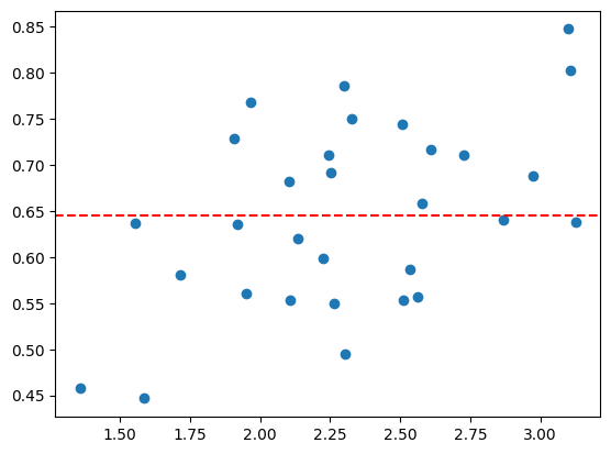
As a diagnostic plot, we recommend plotting the individual correlation parameter estimates against the estimated fSNR.
[8]:
# Get the individual parameter estimates from the individual fits
theta_ind = theta[0] # Get the parameters from the first (and only model)
r_indiv = Mflex_sim.get_correlation(theta[0]) # Inverse fisher-z transform
fSNR_indiv = Mflex_sim.get_fSNR(theta[0], n_part, separate=False)
[9]:
# Add the group estimate as a horizontal line
theta_g,_= pcm.group_to_individ_param(theta_gr[0],Mflex_sim,20)
r_group = Mflex_sim.get_correlation(theta_g)
[10]:
# Make the diagnostic plot of the correlation parameter against the fSNR
plt.scatter(fSNR_indiv, r_indiv)
plt.axhline(r_group[0], color='red', linestyle='--')
plt.axhline(1, color='k', linestyle=':')
plt.axhline(-1, color='k', linestyle=':')
plt.axhline(0, color='k', linestyle=':')
plt.xlabel('fSNR')
plt.ylabel('Correlation parameter')
[10]:
Text(0, 0.5, 'Correlation parameter')
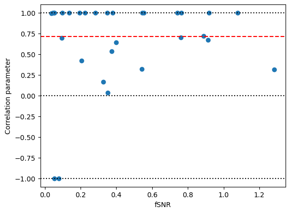
The Figure show the individual correlation estimates plotted against the fSNR, As we can see, the group estimate (red line) is quite close to the true (simulated) value. Individual estimates show a downward bias that and increased variance that becomes worse as the fSNR decreases. Correlation estimates also increasingly hit the boundaries of -1 and 1 as the fSNR decreases.
One-sample inference via bootstrap
To test whether the estimated group correlation is smaller than a specific value (for example true_corr=1, indicating that the activity patterns are the same), we can use a group bootstrap. In this approach, we resample the datasets (participants) with replacement, and for each resampled dataset, we calculate the group correlation estimate. This gives us a distribution of group correlation estimates. If the hypothesized value (x) is outside the 95% confidence interval (for a two-sided test)
or 90% confidence interval (for a one-sided test) we can reject the hypothesis that r = x.
[11]:
r_boot,fSNR_boot,_ = pcm.bootstrap_group_corr(D,Mflex_sim,fixed_effect=None,n_bootstr=200,verbose=True)
Bootstrapping 200 samples:
Bootstrap sample 0/200
Bootstrap sample 50/200
Bootstrap sample 100/200
Bootstrap sample 150/200
[12]:
ax=sns.stripplot(y=r_boot,dodge=True,legend=False)
ax.set_ylim([0,1.05])
x_coord = ax.get_xticks()
CI_low = np.percentile(r_boot, 2.5)
CI_high = np.percentile(r_boot, 97.5)
pcm.plot_CI(ax,x_coord[0],center=r_group,low=CI_low,high=CI_high,width=0.2,facecolor='black',alpha=0.3)
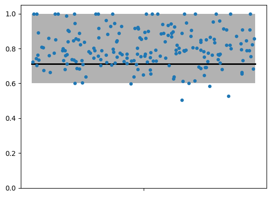
The Figure shows the distribution of the group correlation estimates obtained from the bootstrap procedure. The black line indicates the group estimate obtained from the original data, and the shaded area indicates the 95% confidence interval obtained from the bootstrap distribution. As we can see, the true value of 0.7 is well within the confidence interval, so we cannot reject the hypothesis that r = 0.7. However, if we had hypothesized that r = 1, we would have been able to reject this hypothesis, as 1 is outside the confidence interval. Note the the lower bound of the confidence interval tends to be a bit too high, so testing whether r is larger than a specific value needs to be done with caution (Diedrichsen et al., 2026).
Paired-sample inference via bootstrap
We can extend this bootstrap approach to test whether the correlation is higher in one brain area than another. In this case, we fit a separate models for each brain area. For the boostrap procedure, we resample the datasets (participants) with replacement, and for each resampled dataset, we calculate the group correlation estimate for both brain areas. This gives us a distribution of the difference in group correlation estimates between the two brain areas.
[13]:
n_subj = 30
rng = np.random.default_rng(seed=102)
# Data set for brain area 1 with low signal
signal = np.random.gamma(shape=2,scale=0.03,size=(n_subj,))
D1 = pcm.sim.make_dataset(model=Mtrue_sim, \
    theta=[0,0], \
    cond_vec=cond_vec, \
    part_vec=part_vec, \
    n_sim=n_subj, \
    signal=signal,\
    rng=rng)
# Data set for brain area 2 with higher signal, but lower correlation
Mtrue_sim = pcm.CorrelationModel('corr', num_items=1, corr=0.5, cond_effect=False)
signal = np.random.gamma(shape=2,scale=0.08,size=(n_subj,))
D2 = pcm.sim.make_dataset(model=Mtrue_sim, \
    theta=[0,0], \
    cond_vec=cond_vec, \
    part_vec=part_vec, \
    n_sim=n_subj, \
    signal=signal,\
    rng=rng)
[14]:
# Get the group estimates for the two areas and compare the estimated correlation parameters:
T_gr1, theta_gr1 = pcm.fit_model_group(D1, Mflex_sim, fixed_effect=None, fit_scale=True, verbose=False)
theta_g1,_= pcm.group_to_individ_param(theta_gr1[0],Mflex_sim,n_subj)
r_group1 = Mflex_sim.get_correlation(theta_g1).mean()
fSNR_group1 = Mflex_sim.get_fSNR(theta_g1, n_part, separate=False).mean()
T_gr2, theta_gr2 = pcm.fit_model_group(D2, Mflex_sim, fixed_effect=None, fit_scale=True, verbose=False)
theta_g2,_= pcm.group_to_individ_param(theta_gr2[0],Mflex_sim,n_subj)
r_group2 = Mflex_sim.get_correlation(theta_g2).mean()
fSNR_group2 = Mflex_sim.get_fSNR(theta_g2, n_part, separate=False).mean()
print(f"Estimated group correlation for the different areas are: {r_group1:.4f} , {r_group2:.4f}")
print(f"Estimated fSNR  for the different areas are: {fSNR_group1:.4f} , {fSNR_group2:.4f}")
Estimated group correlation for the different areas are: 0.8293 , 0.4975
Estimated fSNR  for the different areas are: 0.2947 , 1.0843
Note that the fSNR is much lower for the first dataset, so if we calculated Pearson correlations, we would have concluded that the correlation is higher in the second dataset. However, when we take into account the measurement noise, we see that the estimated group correlation is actually higher for the first dataset.
To test this hypothesis we are running the bootstrap for each dataset. The bootstrap for the second dataset will be done with the same bootstrap indices than for the first dataset. We can use the distribution of the difference in correlation of those paired bootstrap samples to test whether the correlation of D1 > D2.
[15]:
r_boot1,fSNR_boot1,boot_indx = pcm.bootstrap_group_corr(D1,Mflex_sim,fixed_effect=None,n_bootstr=200,verbose=True)
r_boot2,fSNR_boot2,boot_indx = pcm.bootstrap_group_corr(D2,Mflex_sim,fixed_effect=None,n_bootstr=200,verbose=True,boot_indx=boot_indx)
diff_boot = r_boot1 - r_boot2
Bootstrapping 200 samples:
Bootstrap sample 0/200
Bootstrap sample 50/200
Bootstrap sample 100/200
Bootstrap sample 150/200
Bootstrapping 200 samples:
Bootstrap sample 0/200
Bootstrap sample 50/200
Bootstrap sample 100/200
Bootstrap sample 150/200
[16]:
CI_low = np.percentile(diff_boot, 2.5)
CI_high = np.percentile(diff_boot, 97.5)
print(f"95% confidence interval for the difference in correlation is: [{CI_low:.4f}, {CI_high:.4f}]")
95% confidence interval for the difference in correlation is: [0.1322, 0.4859]
Given these results, we can conclude that the correlation in D1 is significantly different from D2.
Multi-pattern setting: Estimating the correlation between two sets of patterns across two conditions
In the second part of this notebook, we will simulate data from a hypothetical experiment, in which participants observed 3 hand gestures or executed the same 3 hand gestures. Thus, we have 3 items (i.e., the hand gestures) in each of 2 conditions (i.e., either observe or execute).
We are interested in the average correlation between the patterns associated with observing and executing action A, observing and executing action B, and observing and executing action C, while accounting for overall differences in the average patterns of observing and executing.
For the condition effect, we have two options: We can either model the condition effect as a random effect with an associated pattern variance. We will take this approach when generating the data. We can also model the condition effect as a fixed effect, which is equivalent to removing the mean pattern for each condition from the data - this approach is taken here when fitting the model.
Simulating data
First, we create our true model (Mtrue): one where the all actions are equally strongly encoded in each condition, but where the strength of encoding can differ between conditions (i.e., between observation or execution).
For example, we could expect the difference between actions to be smaller during observation than during execution (simply due to overall levels of brain activation).
Next, we also model the covariance between items within each condition with a condition effect (i.e., by setting condEffect to True). Finally, we set the ground-truth correlation to be 0.7.
[17]:
Mtrue = pcm.CorrelationModel('corr', num_items=3, corr=0.7, cond_effect=True, within_cov=None)
print(f"The true model has {Mtrue.n_param} hyper parameters")
The true model has 4 hyper parameters
These four parameters are concerned with the condition effect and item effect for observation and execution, respectively. Visualizing the components of the second moment matrix (also known as variance-covariance, or simply covariance matrix) helps to understand this:
[18]:
H = Mtrue.n_param
for i in range(H):
    plt.subplot(1, H, i+1)
    plt.imshow(Mtrue.Gc[i,:,:])
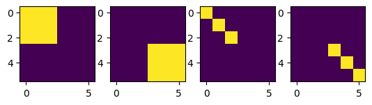
The first two components plotted above reflect the condition effect and model the covariance between items within each condition (observation, execution). The second two components reflect the item effect and model the item-specific variance for each item (3 hand gestures) in each condition.
To Simulate a dataset, we need to simulate an experimental design. Let’s assume we measure the 6 trial types (3 items x 2 conditions) in 8 imaging runs and submit the beta-values from each run to the model as \(\mathbf{Y}\).
We then generate a dataset where there is a strong overall effect for both observation (exp(0)) and execution (exp(1)). In comparison, the item-specific effects for observation (exp(-1.5)) and execution (exp(-1)) are pretty weak (this is a rather typical for real fMRI data).
Note that all hyper parameters are log(variances) — this ensures that the variances positive and the math easy.
[19]:
# Create the design. In this case it's 8 runs, 6 trial types
n_part = 8
cond_vec, part_vec = pcm.sim.make_design(n_cond=6, n_part=n_part)
#print(cond_vec)
#print(part_vec)

# Starting from the true model above, generate 20 datasets/participants
theta_true = [0,1,-1.5,-1]
D = pcm.sim.make_dataset(model=Mtrue, \
    theta=theta_true, \
    cond_vec=cond_vec, \
    part_vec=part_vec, \
    n_sim=n_subj, \
    signal=1)
Inspecting the data
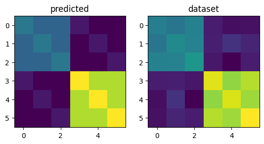
As a quick check, let’s plot the predicted second moment matrix of our true model (using the simulation parameters) and the crossvalidated estimate from the first dataset.
[20]:
# Get the predicted G-matrix  from the true model
G,_ = Mtrue.predict([0,1,-1.5,-1])

# The estimated G-matrix from the first dataset
trial_type = D[1].obs_descriptors['cond_vec']
G_hat,_ = pcm.est_G_crossval(D[1].measurements, trial_type, part_vec)

# Visualize the second moment (G) matrices
plt.subplot(1,2,1)
plt.imshow(G)
plt.title('predicted')

plt.subplot(1,2,2)
plt.imshow(G_hat)
plt.title('dataset')
[20]:
Text(0.5, 1.0, 'dataset')
Fitting models
We now use a flexible correlation model (Mflex). In this case we do not want to model the condition as random effect, as we are removing them as a fixed effect when fitting the model.
[21]:
# Now make the flexible model without a condition effect (given that we are removing the condition effect as a fixed effect when fitting the model).
Mflex = pcm.CorrelationModel("flex", num_items=3, corr=None, cond_effect=False)
print(f"The true model has {Mflex.n_param} hyper parameters")
The true model has 3 hyper parameters
We can now fit the model to the datasets in one go. The resulting dataframe T has the log-likelihoods for each model (columns) / dataset (rows). The second return argument theta contains the parameters for each model fit.
[22]:
# If we want to remove the condition effect as a fixed effect, we need an indicator for that
c_vec,item_vec= pcm.cond_to_item(cond_vec)
X = pcm.matrix.indicator(c_vec)
[23]:
T, theta = pcm.fit_model_individ(D, Mflex, fixed_effect=X, fit_scale=False, verbose=False)
T.head()
[23]:
| variable | likelihood | noise | iterations |
|---|---|---|---|
| model | flex | flex | flex |
| 0 | -867.481383 | 1.013683 | 5.0 |
| 1 | -789.748201 | 0.914802 | 5.0 |
| 2 | -867.886292 | 1.024330 | 5.0 |
| 3 | -834.834155 | 0.987000 | 5.0 |
| 4 | -832.124485 | 0.982413 | 5.0 |
[24]:
# Now the group fit
T_gr, theta_gr = pcm.fit_model_group(D, Mflex, fixed_effect=X, fit_scale=False, verbose=False)
T_gr.head()
[24]:
| variable | likelihood | noise | scale | iterations |
|---|---|---|---|---|
| model | flex | flex | flex | flex |
| 0 | -870.684370 | 1.015143 | 0.0 | 5 |
| 1 | -790.229614 | 0.913811 | 0.0 | 5 |
| 2 | -868.271846 | 1.023243 | 0.0 | 5 |
| 3 | -836.538227 | 0.985193 | 0.0 | 5 |
| 4 | -833.775346 | 0.978006 | 0.0 | 5 |
Interpreting the model fits
Again, the key diagnostic plot is to look at the ML estimates of the parameters against the overall SNR. Note that the first two parameters are the main condition effects
[25]:
# Plot individual parameter estimates against the individual noise level
r_indiv = Mflex.get_correlation(theta[0])
fSNR_indiv = Mflex.get_fSNR(theta[0], n_part, separate=False)
plt.scatter(fSNR_indiv, r_indiv)

# Add the group estimate as a horizontal line
theta_g,_= pcm.group_to_individ_param(theta_gr[0],Mflex,n_subj)
r_group = Mflex.get_correlation(theta_g)
plt.axhline(r_group[0], color='red', linestyle='--')
[25]:
<matplotlib.lines.Line2D at 0x177dc5b10>
Inference via bootstrap
Again, we can use the bootstrap to get confidence intervals for the group-level correlation parameter In this case we need to specify the fixed (condition) effects. For this example we draw 200 bootstrap samples-in practice we recommend 5000 or more.
[26]:
r_boot,fSNR_boot,_ = pcm.bootstrap_group_corr(D,Mflex,fixed_effect=X,n_bootstr=200,verbose=True)
Bootstrapping 200 samples:
Bootstrap sample 0/200
Bootstrap sample 50/200
Bootstrap sample 100/200
Bootstrap sample 150/200
[27]:
# From the bootstrap samples, we can get an approximate confidence interval using the bootstrap method.
CI_low = np.percentile(r_boot, 2.5)
CI_high = np.percentile(r_boot, 97.5)
print(f"95% confidence interval for the group-level correlation parameter: [{CI_low:.3f}, {CI_high:.3f}]")
95% confidence interval for the group-level correlation parameter: [0.609, 0.685]